4.8 KiB
MATH 6601 - Project 1 Report
Author: Zhe Yuan (yuan.1435)
Date: Sep 2025
1. Projections
(a)
The projection of vector b onto the column space of a full-rank matrix A is given by p=A(A^*A)^{-1}A^*b. A function proj(A, b) was implemented based on this formula (see Project1_Q1.py). For \epsilon = 1, the projection is:
p ≈ [1.85714286, 1.0, 3.14285714, 1.28571429, 3.85714286]
(b)
As \epsilon \rightarrow 0, the normal equation method numerically unstable. A more robust SVD-based method, proj_SVD(A, b), was implemented to handle this (see Project1_Q1.py).
Results:
\epsilon |
Normal Equation Method proj(A, b) |
SVD Method proj_SVD(A, b) |
Difference (Normal Eq - SVD) |
|---|---|---|---|
| 1.0 | [1.85714286 1. 3.14285714 1.28571429 3.85714286] |
[1.85714286 1. 3.14285714 1.28571429 3.85714286] |
[ 2.22e-16 1.55e-15 -4.44e-16 2.22e-16 -8.88e-16] |
| 0.1 | [1.85714286 1. 3.14285714 1.28571429 3.85714286] |
[1.85714286 1. 3.14285714 1.28571429 3.85714286] |
[ 8.08e-14 5.87e-14 -8.88e-16 4.82e-14 -1.38e-14] |
| 0.01 | [1.85714286 1. 3.14285714 1.28571429 3.85714286] |
[1.85714286 1. 3.14285714 1.28571429 3.85714286] |
[-4.77e-12 -1.84e-14 5.54e-13 -4.00e-12 1.50e-12] |
| 1e-4 | [1.85714282 1. 3.14285716 1.28571427 3.85714291] |
[1.85714286 1. 3.14285714 1.28571429 3.85714286] |
[-3.60e-08 9.11e-13 1.94e-08 -1.20e-08 4.80e-08] |
| 1e-8 | [-1.87500007 0.99999993 -3.12499997 -2.62500007 3.49999996] |
[1.85714286 1. 3.14285714 1.28571427 3.85714286] |
[-3.73e+00 -7.45e-08 -6.27e+00 -3.91e+00 -3.57e-01] |
| 1e-16 | Error: ValueError: Matrix A must be full rank |
[3.4 1. 1.6 1.8 1.8] |
Could not compute difference due to previous error. |
| 1e-32 | Error: ValueError: Matrix A must be full rank |
[3.4 1. 1.6 1.8 1.8] |
Could not compute difference due to previous error. |
Numerical experiments show that as \epsilon becomes small, the difference between the two methods increases. When \epsilon becomes very small (e.g., 1e-8), the normal equation method can't give a valid result and fails when \epsilon continues to decrease (e.g., 1e-16), while the SVD method continues to provide a stable solution.
2. QR Factorisation
(a, b, c)
Four QR factorization algorithms were implemented to find an orthonormal basis Q for the column space of the n \times n Hilbert matrix (for n=2 to 20):
- Classical Gram-Schmidt (CGS,
cgs_q) - Modified Gram-Schmidt (MGS,
mgs_q) - Householder QR (
householder_q) - Classical Gram-Schmidt Twice (CGS-Twice,
cgs_twice_q)
For implementation details, please see the Project1_Q2.py file.
(d)
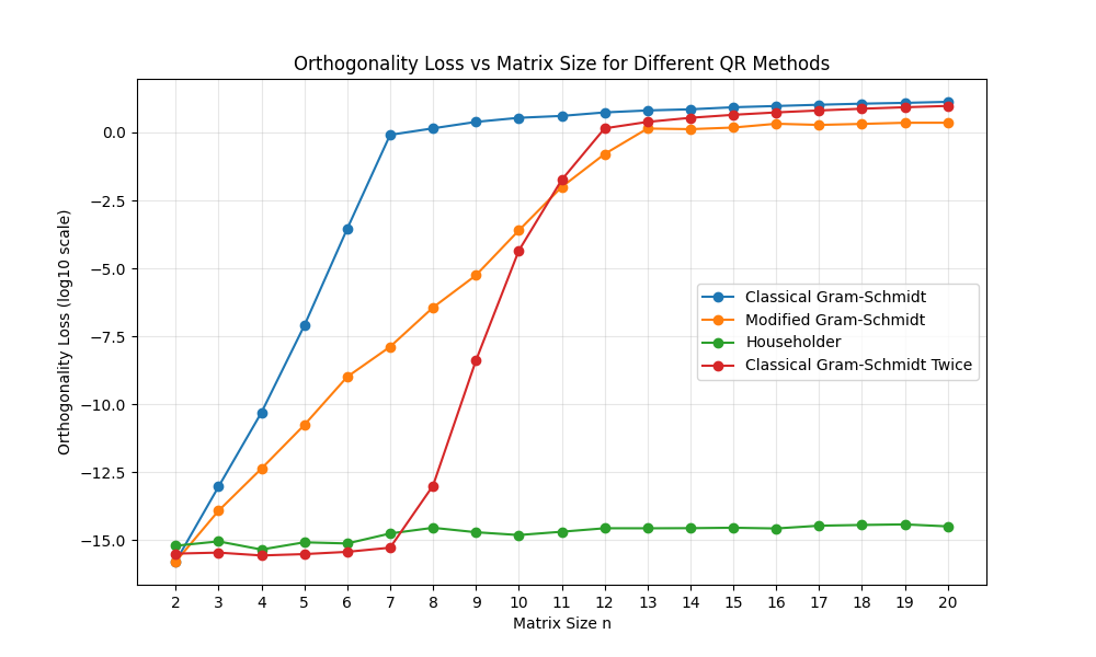
The quality of the computed Q from each method was assessed by plotting the orthogonality loss, log_{10}(||I - Q^T Q||_F), versus the matrix size n.
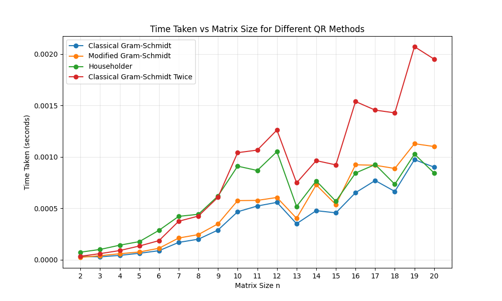
A summary of the loss and computation time for n = 4, 9, 11 is provided below.
(e) The speed and accuracy of the four methods were compared based on the plots.
- Accuracy: Householder is the most accurate and stable. MGS is significantly better than CGS. CGS-Twice improves on CGS, achieving accuracy comparable to MGS. CGS is highly unstable and loses orthogonality quickly.
- Speed: CGS and MGS are the fastest. Householder is slightly slower, and CGS-Twice is the slowest.
3. Least Square Problem
(a)
The problem is formulated as Ax = b, where A is an (N+1) \times (n+1) vandermonde matrix, x is the (n+1) \times 1 vector of unknown polynomial coefficients [a_0, ..., a_n]^T, and b is the (N+1) \times 1 vector of known function values f(t_j).
(b)
The least squares problem was solved using the implemented Householder QR factorization (householder_lstsq in Project1_Q3.py, the same function in Question 2) to find the coefficient vector x.
(c)
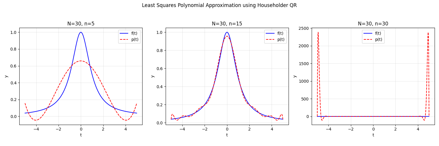
The function f(t) = 1 / (1 + t^2) and its polynomial approximation p(t) were plotted for N=30 and n=5, 15, 30.
When n=15, the approximation is excellent. When n=30, the polynomial interpolates the points but exhibits wild oscillations between them.
(d)
No, p(t) will not converge to f(t) if N = n tends to infinity. Polynomial interpolation on equally spaced nodes diverges for this function, as demonstrated by the severe oscillations in the n=30 case.
(e)
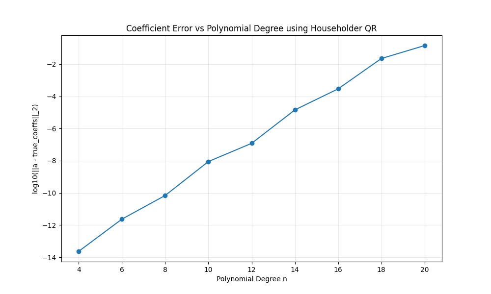
The error between the computed and true coefficients was plotted against the polynomial degree n.
The error in the computed coefficients grows significantly as n increases.


